Deep Reinforcement Learning
Dynamic Programming
Professur für Künstliche Intelligenz - Fakultät für Informatik
Dynamic Programming (DP)
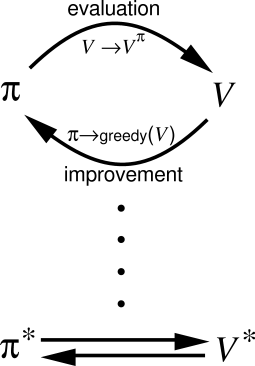
Dynamic Programming (DP) iterates over two steps:
Policy evaluation
- For a given policy \pi, the value of all states V^\pi(s) or all state-action pairs Q^\pi(s, a) is calculated based on the Bellman equations:
V^{\pi} (s) = \sum_{a \in \mathcal{A}(s)} \pi(s, a) \, \sum_{s' \in \mathcal{S}} p(s' | s, a) \, [ r(s, a, s') + \gamma \, V^{\pi} (s') ]
Policy improvement
- From the current estimated values V^\pi(s) or Q^\pi(s, a), a new better policy \pi is derived.
\pi' \leftarrow \text{Greedy}(V^\pi)
After enough iterations, the policy converges to the optimal policy (if the states are Markov).
Two main algorithms: policy iteration and value iteration.
1 - Policy iteration
Policy evaluation
- Bellman equation for the state s and a fixed policy \pi:
V^{\pi} (s) = \sum_{a \in \mathcal{A}(s)} \pi(s, a) \, \sum_{s' \in \mathcal{S}} p(s' | s, a) \, [ r(s, a, s') + \gamma \, V^{\pi} (s') ]
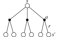
- Let’s note \mathcal{P}_{ss'}^\pi the transition probability between s and s' (dependent on the policy \pi) and \mathcal{R}_{s}^\pi the expected reward in s (also dependent):
\mathcal{P}_{ss'}^\pi = \sum_{a \in \mathcal{A}(s)} \pi(s, a) \, p(s' | s, a)
\mathcal{R}_{s}^\pi = \sum_{a \in \mathcal{A}(s)} \pi(s, a) \, \sum_{s' \in \mathcal{S}} \, p(s' | s, a) \ r(s, a, s')
The Bellman equation becomes V^{\pi} (s) = \mathcal{R}_{s}^\pi + \gamma \, \displaystyle\sum_{s' \in \mathcal{S}} \, \mathcal{P}_{ss'}^\pi \, V^{\pi} (s')
As we have a fixed policy during the evaluation (MRP), the Bellman equation is simplified.
Policy evaluation
- Let’s now put the Bellman equations in a matrix-vector form.
V^{\pi} (s) = \mathcal{R}_{s}^\pi + \gamma \, \sum_{s' \in \mathcal{S}} \, \mathcal{P}_{ss'}^\pi \, V^{\pi} (s')
- We first define the vector of state values \mathbf{V}^\pi:
\mathbf{V}^\pi = \begin{bmatrix} V^\pi(s_1) \\ V^\pi(s_2) \\ \vdots \\ V^\pi(s_n) \\ \end{bmatrix}
- and the vector of expected reward \mathbf{R}^\pi:
\mathbf{R}^\pi = \begin{bmatrix} \mathcal{R}^\pi(s_1) \\ \mathcal{R}^\pi(s_2) \\ \vdots \\ \mathcal{R}^\pi(s_n) \\ \end{bmatrix}
- The state transition matrix \mathcal{P}^\pi is defined as:
\mathcal{P}^\pi = \begin{bmatrix} \mathcal{P}_{s_1 s_1}^\pi & \mathcal{P}_{s_1 s_2}^\pi & \ldots & \mathcal{P}_{s_1 s_n}^\pi \\ \mathcal{P}_{s_2 s_1}^\pi & \mathcal{P}_{s_2 s_2}^\pi & \ldots & \mathcal{P}_{s_2 s_n}^\pi \\ \vdots & \vdots & \vdots & \vdots \\ \mathcal{P}_{s_n s_1}^\pi & \mathcal{P}_{s_n s_2}^\pi & \ldots & \mathcal{P}_{s_n s_n}^\pi \\ \end{bmatrix}
Policy evaluation
- You can simply check that:
\begin{bmatrix} V^\pi(s_1) \\ V^\pi(s_2) \\ \vdots \\ V^\pi(s_n) \\ \end{bmatrix} = \begin{bmatrix} \mathcal{R}^\pi(s_1) \\ \mathcal{R}^\pi(s_2) \\ \vdots \\ \mathcal{R}^\pi(s_n) \\ \end{bmatrix} + \gamma \, \begin{bmatrix} \mathcal{P}_{s_1 s_1}^\pi & \mathcal{P}_{s_1 s_2}^\pi & \ldots & \mathcal{P}_{s_1 s_n}^\pi \\ \mathcal{P}_{s_2 s_1}^\pi & \mathcal{P}_{s_2 s_2}^\pi & \ldots & \mathcal{P}_{s_2 s_n}^\pi \\ \vdots & \vdots & \vdots & \vdots \\ \mathcal{P}_{s_n s_1}^\pi & \mathcal{P}_{s_n s_2}^\pi & \ldots & \mathcal{P}_{s_n s_n}^\pi \\ \end{bmatrix} \times \begin{bmatrix} V^\pi(s_1) \\ V^\pi(s_2) \\ \vdots \\ V^\pi(s_n) \\ \end{bmatrix}
leads to the same equations as:
V^{\pi} (s) = \mathbf{R}_{s}^\pi + \gamma \, \sum_{s' \in \mathcal{S}} \, \mathcal{P}_{ss'}^\pi \, V^{\pi} (s')
for all states s.
- The Bellman equations for all states s can therefore be written with a matrix-vector notation as:
\mathbf{V}^\pi = \mathbf{R}^\pi + \gamma \, \mathcal{P}^\pi \, \mathbf{V}^\pi
Policy evaluation
- The Bellman equations for all states s is:
\mathbf{V}^\pi = \mathbf{R}^\pi + \gamma \, \mathcal{P}^\pi \, \mathbf{V}^\pi
- If we know \mathcal{P}^\pi and \mathbf{R}^\pi (dynamics of the MDP for the policy \pi), we can simply obtain the state values:
(\mathbb{I} - \gamma \, \mathcal{P}^\pi ) \times \mathbf{V}^\pi = \mathbf{R}^\pi
where \mathbb{I} is the identity matrix, what gives:
\mathbf{V}^\pi = (\mathbb{I} - \gamma \, \mathcal{P}^\pi )^{-1} \times \mathbf{R}^\pi
Done!
But, if we have n states, the matrix \mathcal{P}^\pi has n^2 elements.
Inverting \mathbb{I} - \gamma \, \mathcal{P}^\pi requires at least \mathcal{O}(n^{2.37}) operations.
Forget it if you have more than a thousand states (1000^{2.37} \approx 13 million operations).
In dynamic programming, we will use iterative methods to estimate \mathbf{V}^\pi.
Iterative policy evaluation
- The idea of iterative policy evaluation (IPE) is to consider a sequence of consecutive state-value functions which should converge from initially wrong estimates V_0(s) towards the real state-value function V^{\pi}(s).
V_0 \rightarrow V_1 \rightarrow V_2 \rightarrow \ldots \rightarrow V_k \rightarrow V_{k+1} \rightarrow \ldots \rightarrow V^\pi
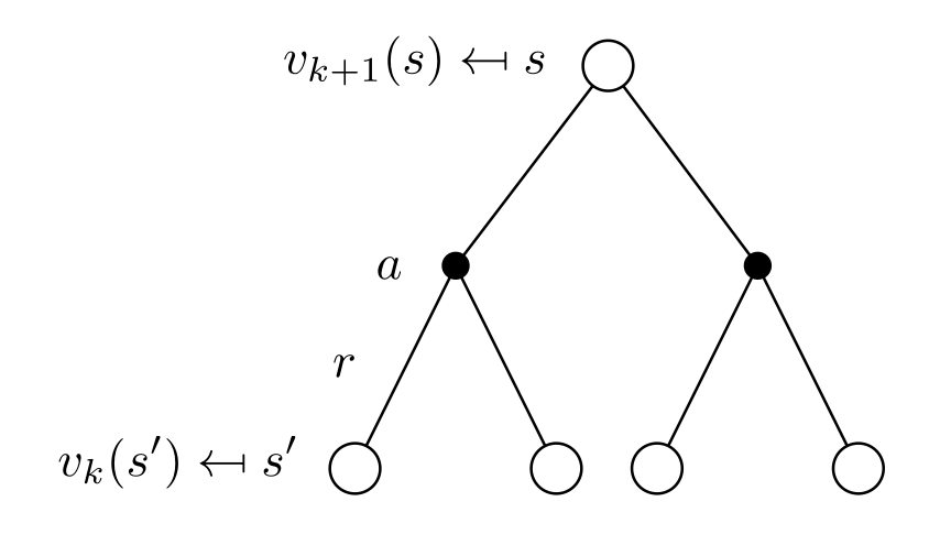
The value function at step k+1 V_{k+1}(s) is computed using the previous estimates V_{k}(s) and the Bellman equation transformed into an update rule.
In vector notation:
\mathbf{V}_{k+1} = \mathbf{R}^\pi + \gamma \, \mathcal{P}^\pi \, \mathbf{V}_k
Iterative policy evaluation
Let’s start with dummy (e.g. random) initial estimates V_0(s) for the value of every state s.
We can obtain new estimates V_1(s) which are slightly less wrong by applying once the Bellman operator:
V_{1} (s) \leftarrow \sum_{a \in \mathcal{A}(s)} \pi(s, a) \, \sum_{s' \in \mathcal{S}} p(s' | s, a) \, [ r(s, a, s') + \gamma \, V_0 (s') ] \quad \forall s \in \mathcal{S}
- Based on these estimates V_1(s), we can obtain even better estimates V_2(s) by applying again the Bellman operator:
V_{2} (s) \leftarrow \sum_{a \in \mathcal{A}(s)} \pi(s, a) \, \sum_{s' \in \mathcal{S}} p(s' | s, a) \, [ r(s, a, s') + \gamma \, V_1 (s') ] \quad \forall s \in \mathcal{S}
- Generally, state-value function estimates are improved iteratively through:
V_{k+1} (s) \leftarrow \sum_{a \in \mathcal{A}(s)} \pi(s, a) \, \sum_{s' \in \mathcal{S}} p(s' | s, a) \, [ r(s, a, s') + \gamma \, V_k (s') ] \quad \forall s \in \mathcal{S}
- V_\infty = V^{\pi} is a fixed point of this update rule because of the uniqueness of the solution to the Bellman equation.
Bellman operator
- The Bellman operator \mathcal{T}^\pi is a mapping between two vector spaces:
\mathcal{T}^\pi (\mathbf{V}) = \mathbf{R}^\pi + \gamma \, \mathcal{P}^\pi \, \mathbf{V}
If you apply repeatedly the Bellman operator on any initial vector \mathbf{V}_0, it converges towards the solution of the Bellman equations \mathbf{V}^\pi.
Mathematically speaking, \mathcal{T}^\pi is a \gamma-contraction, i.e. it makes value functions closer by at least \gamma:
|| \mathcal{T}^\pi (\mathbf{V}) - \mathcal{T}^\pi (\mathbf{U})||_\infty \leq \gamma \, ||\mathbf{V} - \mathbf{U} ||_\infty
The contraction mapping theorem ensures that \mathcal{T}^\pi converges to an unique fixed point:
- Existence and uniqueness of the solution of the Bellman equations.
Backup diagram of IPE
- Iterative Policy Evaluation relies on full backups: it backs up the value of ALL possible successive states into the new value of a state.
V_{k+1} (s) \leftarrow \sum_{a \in \mathcal{A}(s)} \pi(s, a) \, \sum_{s' \in \mathcal{S}} p(s' | s, a) \, [ r(s, a, s') + \gamma \, V_k (s') ] \quad \forall s \in \mathcal{S}
- Backup diagram: which other values do you need to know in order to update one value?
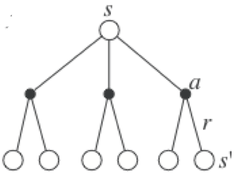
- The backups are synchronous: all states are backed up in parallel.
\mathbf{V}_{k+1} = \mathbf{R}^\pi + \gamma \, \mathcal{P}^\pi \, \mathbf{V}_k
The termination of iterative policy evaluation has to be controlled by hand, as the convergence of the algorithm is only at the limit.
It is good practice to look at the variations on the values of the different states, and stop the iteration when this variation falls below a predefined threshold.
Iterative policy evaluation
For a fixed policy \pi, initialize V(s)=0 \; \forall s \in \mathcal{S}.
while not converged:
for all states s:
- V_\text{target}(s) = \sum_{a \in \mathcal{A}(s)} \pi(s, a) \, \sum_{s' \in \mathcal{S}} p(s' | s, a) \, [ r(s, a, s') + \gamma \, V (s') ]
\delta =0
for all states s:
\delta = \max(\delta, |V(s) - V_\text{target}(s)|)
V(s) = V_\text{target}(s)
if \delta < \delta_\text{threshold}:
- converged = True
Dynamic Programming (DP)

Dynamic Programming (DP) iterates over two steps:
Policy evaluation
- For a given policy \pi, the value of all states V^\pi(s) or all state-action pairs Q^\pi(s, a) is calculated based on the Bellman equations:
V^{\pi} (s) = \sum_{a \in \mathcal{A}(s)} \pi(s, a) \, \sum_{s' \in \mathcal{S}} p(s' | s, a) \, [ r(s, a, s') + \gamma \, V^{\pi} (s') ]
Policy improvement
- From the current estimated values V^\pi(s) or Q^\pi(s, a), a new better policy \pi is derived.
Policy improvement
- For each state s, we would like to know if we should deterministically choose an action a \neq \pi(s) or not in order to improve the policy.
- The value of an action a in the state s for the policy \pi is given by:
Q^{\pi} (s, a) = \sum_{s' \in \mathcal{S}} p(s' | s, a) \, [r(s, a, s') + \gamma \, V^{\pi}(s') ]

- If the Q-value of an action a is higher than the one currently selected by the deterministic policy:
Q^{\pi} (s, a) > Q^{\pi} (s, \pi(s)) = V^{\pi}(s)
then it is better to select a once in s and thereafter follow \pi.
If there is no better action, we keep the previous policy for this state.
This corresponds to a greedy action selection over the Q-values, defining a deterministic policy \pi(s):
\pi(s) \leftarrow \text{argmax}_a \, Q^{\pi} (s, a) = \sum_{s' \in \mathcal{S}} p(s' | s, a) \, [r(s, a, s') + \gamma \, V^{\pi}(s') ]
Policy improvement
- After the policy improvement, the Q-value of each deterministic action \pi(s) has increased or stayed the same.
\text{argmax}_a Q^{\pi} (s, a) = \sum_{s' \in \mathcal{S}} p(s' | s, a) \, [r(s, a, s') + \gamma \, V^{\pi}(s') ] \geq Q^\pi(s, \pi(s))
This defines an improved policy \pi', where all states and actions have a higher value than previously.
Greedy action selection over the state value function implements policy improvement:
\pi' \leftarrow \text{Greedy}(V^\pi)
Greedy policy improvement:
for each state s \in \mathcal{S}:
- \pi(s) \leftarrow \text{argmax}_a \sum_{s' \in \mathcal{S}} p(s' | s, a) \, [r(s, a, s') + \gamma \, V^{\pi}(s') ]
Policy iteration

Once a policy \pi has been improved using V^{\pi} to yield a better policy \pi', we can then compute V^{\pi'} and improve it again to yield an even better policy \pi''.
The algorithm policy iteration successively uses policy evaluation and policy improvement to find the optimal policy.
\pi_0 \xrightarrow[]{E} V^{\pi_0} \xrightarrow[]{I} \pi_1 \xrightarrow[]{E} V^{\pi^1} \xrightarrow[]{I} ... \xrightarrow[]{I} \pi^* \xrightarrow[]{E} V^{*}
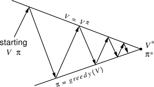
The optimal policy being deterministic, policy improvement can be greedy over the state values.
If the policy does not change after policy improvement, the optimal policy has been found.
Policy iteration
Initialize a deterministic policy \pi(s) and set V(s)=0 \; \forall s \in \mathcal{S}.
while \pi is not optimal:
while not converged: # Policy evaluation
for all states s:
- V_\text{target}(s) = \sum_{a \in \mathcal{A}(s)} \pi(s, a) \, \sum_{s' \in \mathcal{S}} p(s' | s, a) \, [ r(s, a, s') + \gamma \, V (s') ]
for all states s:
- V(s) = V_\text{target}(s)
for each state s \in \mathcal{S}: # Policy improvement
- \pi(s) \leftarrow \text{argmax}_a \sum_{s' \in \mathcal{S}} p(s' | s, a) \, [r(s, a, s') + \gamma \, V^{\pi}(s') ]
if \pi has not changed: break
2 - Value iteration
Value iteration
One drawback of policy iteration is that it uses a full policy evaluation, which can be computationally exhaustive as the convergence of V_k is only at the limit and the number of states can be huge.
The idea of value iteration is to interleave policy evaluation and policy improvement, so that the policy is improved after EACH iteration of policy evaluation, not after complete convergence.
As policy improvement returns a deterministic greedy policy, updating of the value of a state is then simpler:
V_{k+1}(s) = \max_a \sum_{s'} p(s' | s,a) [r(s, a, s') + \gamma \, V_k(s') ]
Note that this is equivalent to turning the Bellman optimality equation into an update rule.
Value iteration converges to V^*, faster than policy iteration, and should be stopped when the values do not change much anymore.
Value iteration
Initialize a deterministic policy \pi(s) and set V(s)=0 \; \forall s \in \mathcal{S}.
while not converged:
for all states s:
- V_\text{target}(s) = \max_a \, \sum_{s' \in \mathcal{S}} p(s' | s, a) \, [ r(s, a, s') + \gamma \, V (s') ]
\delta = 0
for all states s:
\delta = \max(\delta, |V(s) - V_\text{target}(s)|)
V(s) = V_\text{target}(s)
if \delta < \delta_\text{threshold}:
- converged = True
Comparison of Policy- and Value-iteration
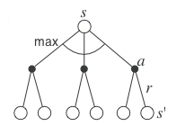
Full policy-evaluation backup
V_{k+1} (s) \leftarrow \sum_{a \in \mathcal{A}(s)} \pi(s, a) \, \sum_{s' \in \mathcal{S}} p(s' | s, a) \, [ r(s, a, s') + \gamma \, V_k (s') ]

Full value-iteration backup
V_{k+1} (s) \leftarrow \max_{a \in \mathcal{A}(s)} \sum_{s' \in \mathcal{S}} p(s' | s, a) \, [ r(s, a, s') + \gamma \, V_k (s') ]
Asynchronous dynamic programming
Synchronous DP requires exhaustive sweeps of the entire state set (synchronous backups).
while not converged:
for all states s:
- V_\text{target}(s) = \max_a \, \sum_{s' \in \mathcal{S}} p(s' | s, a) \, [ r(s, a, s') + \gamma \, V (s') ]
for all states s:
- V(s) = V_\text{target}(s)
Asynchronous DP updates instead each state independently and asynchronously (in-place):
while not converged:
Pick a state s randomly (or following a heuristic).
Update the value of this state.
V(s) = \max_a \, \sum_{s' \in \mathcal{S}} p(s' | s, a) \, [ r(s, a, s') + \gamma \, V (s') ]
We must still ensure that all states are visited, but their frequency and order is irrelevant.
Efficiency of Dynamic Programming

Policy-iteration and value-iteration consist of alternations between policy evaluation and policy improvement, although at different frequencies.
This principle is called Generalized Policy Iteration (GPI).
Finding an optimal policy is polynomial in the number of states and actions: \mathcal{O}(n^2 \, m) (n is the number of states, m the number of actions).
However, the number of states is often astronomical, e.g., often growing exponentially with the number of state variables (what Bellman called “the curse of dimensionality”).
In practice, classical DP can only be applied to problems with a few millions of states.
Curse of dimensionality
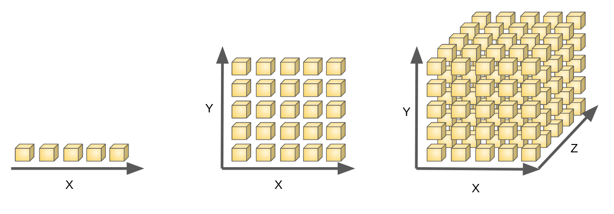
If one variable can be represented by 5 discrete values:
2 variables necessitate 25 states,
3 variables need 125 states, and so on…
The number of states explodes exponentially with the number of dimensions of the problem.