Deep Reinforcement Learning
Advantage actor-critic (A2C, A3C)
Professur für Künstliche Intelligenz - Fakultät für Informatik
1 - Advantage actor-critic
Advantage actor-critic
- Let’s consider an n-step actor-critic architecture where the Q-value of the action (s_t, a_t) is approximated by the n-step return:
Q^{\pi_\theta}(s_t, a_t) \approx R_t^n = \sum_{k=0}^{n-1} \gamma^{k} \, r_{t+k+1} + \gamma^n \, V_\varphi(s_{t+n})
- The actor \pi_\theta(s, a) uses PG with baseline to learn the policy:
\nabla_\theta \mathcal{J}(\theta) = \mathbb{E}_{s_t \sim \rho_\theta, a_t \sim \pi_\theta}[\nabla_\theta \log \pi_\theta (s_t, a_t) \, (R_t^n - V_\varphi(s_t)) ]
- The critic V_\varphi(s) approximates the value of each state:
\mathcal{L}(\varphi) = \mathbb{E}_{s_t \sim \rho_\theta, a_t \sim \pi_\theta}[(R^n_t - V_\varphi(s_t))^2]
Advantage actor-critic
Advantage actor-critic
The advantage actor-critic is strictly on-policy:
The critic must evaluate actions selected the current version of the actor \pi_\theta, not an old version or another policy.
The actor must learn from the current value function V^{\pi_\theta} \approx V_\varphi.
\begin{cases} \nabla_\theta \mathcal{J}(\theta) = \mathbb{E}_{s_t \sim \rho_\theta, a_t \sim \pi_\theta}[\nabla_\theta \log \pi_\theta (s_t, a_t) \, (R^n_t - V_\varphi(s_t)) ] \\ \\ \mathcal{L}(\varphi) = \mathbb{E}_{s_t \sim \rho_\theta, a_t \sim \pi_\theta}[(R^n_t - V_\varphi(s_t))^2] \\ \end{cases}
- We cannot use an experience replay memory to deal with the correlated inputs, as it is only for off-policy methods.
Distributed RL
- We cannot get an uncorrelated batch of transitions by acting sequentially with a single agent.

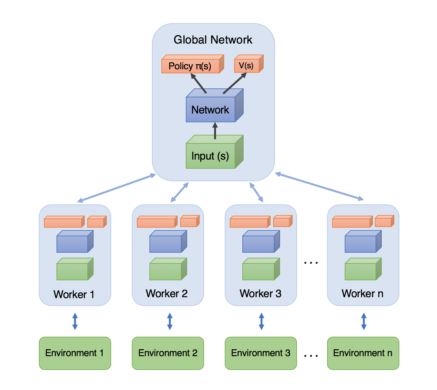
- A simple solution is to have multiple actors with the same weights \theta interacting in parallel with different copies of the environment.
Each rollout worker (actor) starts an episode in a different state: at any point of time, the workers will be in uncorrelated states.
From time to time, the workers all send their experienced transitions to the learner which updates the policy using a batch of uncorrelated transitions.
After the update, the workers use the new policy.
Distributed RL
Distributed RL
Initialize global policy or value network \theta.
Initialize N copies of the environment in different states.
while True:
for each worker in parallel:
- Copy the global network parameters \theta to each worker:
\theta_k \leftarrow \theta
Initialize an empty transition buffer \mathcal{D}_k.
Perform d steps with the worker on its copy of the environment.
Append each transition (s, a, r, s') to the transition buffer.
join(): wait for each worker to terminate.
Gather the N transition buffers into a single buffer \mathcal{D}.
Update the global network on \mathcal{D} to obtain new weights \theta.
Distributed RL for value-based networks (DQN variants)
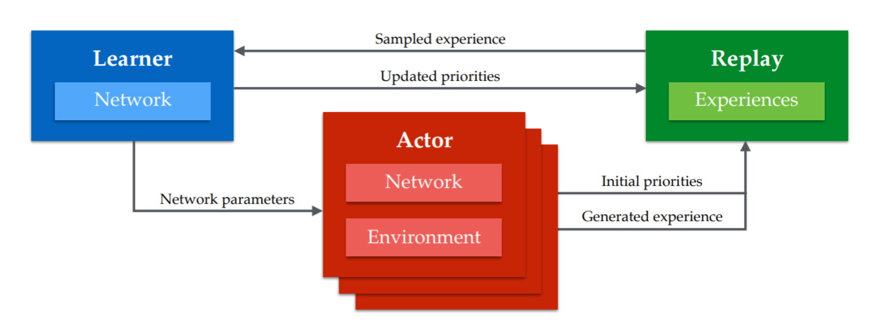
Distributed learning can be used for any deep RL algorithm, including DQN variants.
Distributed DQN variants include GORILA, IMPALA, APE-X, R2D2.
“All” you need is one (or more) GPU for training the global network and N CPU cores for the workers.
The workers fill the ERM much more quickly.
Horgan, D., Quan, J., Budden, D., Barth-Maron, G., Hessel, M., van Hasselt, H., et al. (2018). Distributed Prioritized Experience Replay. arXiv:1803.00933.
Distributed RL
In practice, managing the communication between the workers and the global network through processes can be quite painful.
There are some frameworks abstracting the dirty work, such as RLlib.
Distributed RL
Having multiple workers interacting with different environments is easy in simulation (Atari games).
With physical environments, working in real time, it requires lots of money…
2 - A3C: Asynchronous advantage actor-critic
Mnih, V., Badia, A. P., Mirza, M., Graves, A., Lillicrap, T. P., Harley, T., et al. (2016). Asynchronous Methods for Deep Reinforcement Learning. ICML. arXiv:1602.01783
A3C: Asynchronous advantage actor-critic
Mnih et al. (2016) proposed the A3C algorithm (asynchronous advantage actor-critic).
The stochastic policy \pi_\theta is produced by the actor with weights \theta and learned using :
\nabla_\theta \mathcal{J}(\theta) = \mathbb{E}_{s_t \sim \rho_\theta, a_t \sim \pi_\theta}[\nabla_\theta \log \pi_\theta (s_t, a_t) \, (R^n_t - V_\varphi(s_t)) ]
- The value of a state V_\varphi(s) is produced by the critic with weights \varphi, which minimizes the mse with the n-step return:
\mathcal{L}(\varphi) = \mathbb{E}_{s_t \sim \rho_\theta, a_t \sim \pi_\theta}[(R^n_t - V_\varphi(s_t))^2]
R^n_t = \sum_{k=0}^{n-1} \gamma^{k} \, r_{t+k+1} + \gamma^n \, V_\varphi(s_{t+n})
Both the actor and the critic are trained on batches of transitions collected using parallel workers.
Two things are different from the general distributed approach: workers compute partial gradients and updates are asynchronous.
Mnih, V., Badia, A. P., Mirza, M., Graves, A., Lillicrap, T. P., Harley, T., et al. (2016). Asynchronous Methods for Deep Reinforcement Learning. ICML. arXiv:1602.01783
A3C: Asynchronous advantage actor-critic

def worker(\theta, \varphi):
Initialize empty transition buffer \mathcal{D}. Initialize the environment to the last state visited by this worker.
for n steps:
- Select an action using \pi_\theta, store the transition in the transition buffer.
for each transition in \mathcal{D}:
- Compute the n-step return in each state R^n_t = \displaystyle\sum_{k=0}^{n-1} \gamma^{k} \, r_{t+k+1} + \gamma^n \, V_\varphi(s_{t+n})
Compute policy gradient for the actor on the transition buffer: d\theta = \nabla_\theta \mathcal{J}(\theta) = \frac{1}{n} \sum_{t=1}^n \nabla_\theta \log \pi_\theta (s_t, a_t) \, (R^n_t - V_\varphi(s_t))
Compute value gradient for the critic on the transition buffer: d\varphi = \nabla_\varphi \mathcal{L}(\varphi) = -\frac{1}{n} \sum_{t=1}^n (R^n_t - V_\varphi(s_t)) \, \nabla_\varphi V_\varphi(s_t)
return d\theta, d\varphi
A2C: global networks
Initialize actor \theta and critic \varphi.
Initialize K workers with a copy of the environment.
for t \in [0, T_\text{total}]:
for K workers in parallel:
- d\theta_k, d\varphi_k = worker(\theta, \varphi)
join()
Merge all gradients:
d\theta = \frac{1}{K} \sum_{i=1}^K d\theta_k \; ; \; d\varphi = \frac{1}{K} \sum_{i=1}^K d\varphi_k
- Update the actor and critic using gradient ascent/descent:
\theta \leftarrow \theta + \eta \, d\theta \; ; \; \varphi \leftarrow \varphi - \eta \, d\varphi
A3C: Asynchronous advantage actor-critic
The previous slide depicts A2C, the synchronous version of A3C.
A2C synchronizes the workers (threads), i.e. it waits for the K workers to finish their job before merging the gradients and updating the global networks.
A3C is asynchronous:
the partial gradients are applied to the global networks as soon as they are available.
No need to wait for all workers to finish their job.
As the workers are not synchronized, this means that one worker could be copying the global networks \theta and \varphi while another worker is writing them.
This is called a Hogwild! update: no locks, no semaphores. Many workers can read/write the same data.
It turns out NN are robust enough for this kind of updates.
A3C: asynchronous updates
Initialize actor \theta and critic \varphi.
Initialize K workers with a copy of the environment.
for K workers in parallel:
for t \in [0, T_\text{total}]:
Copy the global networks \theta and \varphi.
Compute partial gradients:
d\theta_k, d\varphi_k = \text{worker}(\theta, \varphi)
- Update the global actor and critic using the partial gradients:
\theta \leftarrow \theta + \eta \, d\theta_k
\varphi \leftarrow \varphi - \eta \, d\varphi_k
A3C: Asynchronous advantage actor-critic

A3C does not use an experience replay memory as DQN.
Instead, it uses multiple parallel workers to distribute learning.
Each worker has a copy of the actor and critic networks, as well as an instance of the environment.
Weight updates are synchronized regularly though a master network using Hogwild!-style updates (every n=5 steps!).
Because the workers learn different parts of the state-action space, the weight updates are not very correlated.
- It works best on shared-memory systems (multi-core) as communication costs between GPUs are huge.
Mnih, V., Badia, A. P., Mirza, M., Graves, A., Lillicrap, T. P., Harley, T., et al. (2016). Asynchronous Methods for Deep Reinforcement Learning. ICML. arXiv:1602.01783
A3C : results
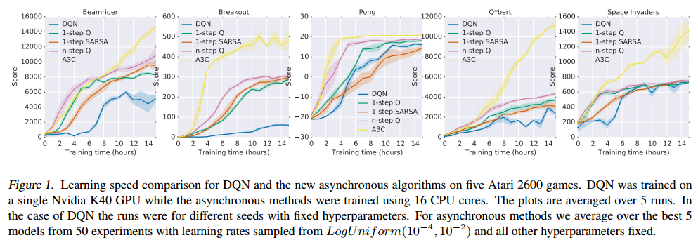
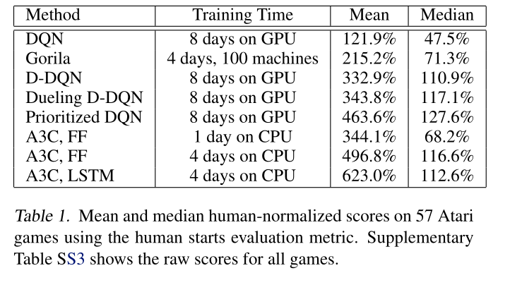
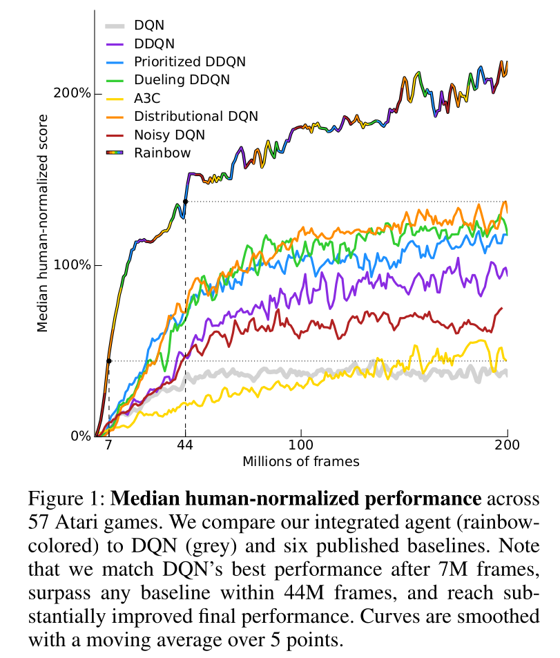
A3C set a new record for Atari games in 2016.
The main advantage is that the workers gather experience in parallel: training is much faster than with DQN.
LSTMs can be used to improve the performance.
Mnih, V., Badia, A. P., Mirza, M., Graves, A., Lillicrap, T. P., Harley, T., et al. (2016). Asynchronous Methods for Deep Reinforcement Learning. ICML. arXiv:1602.01783
A3C : results
- Learning is only marginally better with more threads:

but much faster!

Mnih, V., Badia, A. P., Mirza, M., Graves, A., Lillicrap, T. P., Harley, T., et al. (2016). Asynchronous Methods for Deep Reinforcement Learning. ICML. arXiv:1602.01783
A3C: TORCS simulator
A3C: Labyrinth
A3C: continuous control problems
Comparison with DQN
- A3C came up in 2016. A lot of things happened since then…
